Running Circuits on Hardware

This tutorial shows how a quantum circuit can be run on actual quantum hardware. This requires a valid IBM Quantum Token as well as a service-crn for available quantum backend instances. Please make sure you have sufficient time available to execute the code on the quantum hardware.

Import all Necessary Libraries

from NoisyCircuits.QuantumCircuit import QuantumCircuit as nqc
from NoisyCircuits.utils.CreateNoiseModel import GetNoiseModel
from NoisyCircuits.RunOnHardware import RunOnHardware
import os
import json
import matplotlib.pyplot as plt

2026-03-06 16:05:48,048 INFO util.py:154 -- Missing packages: ['ipywidgets']. Run `pip install -U ipywidgets`, then restart the notebook server for rich notebook output.

Define the Necessary Parameters

api_json = json.load(open(os.path.join(os.path.expanduser("~"), "ibm_api.json"), "r"))
token = api_json["apikey"] # Replace with your Token
service_crn = api_json["service-crn"] # Replace with your Service CRN
backend_name = "ibm_fez"
shots = 1024
verbose = False
jsonize = True
num_qubits = 2
num_trajectories = 100
qpu = "heron" # Only possible option for IBM backends at the moment
num_cores = 4
sim_backend = "pennylane" # Choose between "pennylane", "qiskit" and "qulacs"

Get the Noise Model

noise_model = GetNoiseModel(
    token=token,
    backend_name=backend_name,
    service_crn=service_crn
).get_noise_model()

Warning: Found relaxation time anomaly for qubit 72 with $T_2 \geq 2T_1$. Setting $T_2 = 2T_1$.

Build the Quantum Circuit

For this tutorial, we stick to the simple Bell State circuit

circuit = nqc(num_qubits=num_qubits,
         noise_model=noise_model,
         num_cores=num_cores,
         backend_qpu_type=qpu,
         num_trajectories=num_trajectories,
         sim_backend=sim_backend,
         jsonize=jsonize,
         verbose=verbose)

Successfully switched backend to pennylane.

2026-03-06 16:06:10,852 INFO worker.py:2007 -- Started a local Ray instance.
/Users/adam-ukj7r05xnu2fywx/miniconda3/envs/NoisyCircuits/lib/python3.10/site-packages/ray/_private/worker.py:2046: FutureWarning: Tip: In future versions of Ray, Ray will no longer override accelerator visible devices env var if num_gpus=0 or num_gpus=None (default). To enable this behavior and turn off this error message, set RAY_ACCEL_ENV_VAR_OVERRIDE_ON_ZERO=0
  warnings.warn(

circuit.refresh()
circuit.H(0)
circuit.CX(0, 1)

Perform a Simulation

This is so that we can compare the results of a simulated quantum circuit to actual results from hardware

probs_pure = circuit.run_pure_state(qubits=[0, 1])
probs_simulated = circuit.execute(qubits=[0, 1], num_trajectories=100)

Initialize the Hardware Interface Module

hardware_runner = RunOnHardware(
    token=token,
    backend=backend_name,
    shots=shots
)

qiskit_runtime_service._discover_account:WARNING:2026-03-06 16:06:19,485: Loading account with the given token. A saved account will not be used.
qiskit_runtime_service.__init__:WARNING:2026-03-06 16:06:22,838: Instance was not set at service instantiation. Free and trial plan instances will be prioritized. Based on the following filters: (tags: None, region: us-east, eu-de), and available plans: (open), the available account instances are: Open_Sys. If you need a specific instance set it explicitly either by using a saved account with a saved default instance or passing it in directly to QiskitRuntimeService().
qiskit_runtime_service.backends:WARNING:2026-03-06 16:06:22,840: Loading instance: Open_Sys, plan: open

Submitting the Circuit

Create the low-level circuit instructions for the hardware

hardware_runner.create_circuits(
    circuit=circuit,
    measure_qubits=[0, 1])

Compile the circuit for submission

hardware_runner.setup_circuits()

qiskit_runtime_service.backends:WARNING:2026-03-06 16:06:25,117: Using instance: Open_Sys, plan: open

Submit the circuit to IBM hardware. This returns the unique job id from IBM that can be used to retreive the results.

job_id = hardware_runner.run()

qiskit_runtime_service.backends:WARNING:2026-03-06 16:06:26,641: Using instance: Open_Sys, plan: open

Job ID: d6leqtc3pels739v7um0

[2026-03-06 16:06:41,280 E 415793 416266] core_worker_process.cc:842: Failed to establish connection to the metrics exporter agent. Metrics will not be exported. Exporter agent status: RpcError: Running out of retries to initialize the metrics agent. rpc_code: 14

Retrieve Results from Hardware

results_from_hardware = hardware_runner.get_results(job_id=job_id)
probs_hardware = results_from_hardware[0]

Compare Results

plt.figure(figsize=(12, 5))
x_labels = [f"|{i}{j}\u27E9" for i in range(2) for j in range(2)]
indices = list(range(len(x_labels)))
bar_width = 0.25

plt.bar([i - bar_width for i in indices], probs_pure, width=bar_width, label="Pure State", alpha=0.7, color="C2")
plt.bar(indices, probs_simulated, width=bar_width, label="Simulated", alpha=0.7, color="C0")
plt.bar([i + bar_width for i in indices], probs_hardware, width=bar_width, label="Hardware", alpha=0.7, color="C1")
plt.xticks(indices, x_labels)
plt.xlabel("States", fontsize=14)
plt.ylabel("Probabilities", fontsize=14)
plt.title("Comparison of Simulated vs Hardware Results", fontsize=16)
plt.legend(fontsize=12)
plt.tight_layout()
plt.show()

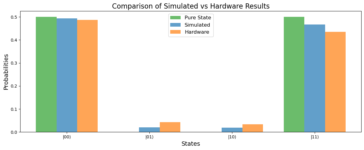
Fidelity with the Battacharyya Coefficient

The Battacharyya Coefficient is a statistical measure of similarity between two probability distributions and is symmetrical. It is given by: \begin{equation} BC(p, q) = \int \sqrt{p\cdot q} \end{equation} and the below equation shows the calculation of the coefficient for two discrete probability distributions: \begin{equation} BC(p, q) = \sum_{i=1}^{N}\sqrt{p_i q_i} \end{equation}

def battacharyya_coefficient(p, q):
    return sum((p_i * q_i) ** 0.5 for p_i, q_i in zip(p, q))

print("Fidelity between Pure State and Simulated:", battacharyya_coefficient(probs_pure, probs_simulated))
print("Fidelity between Pure State and Hardware:", battacharyya_coefficient(probs_pure, probs_hardware))
print("Fidelity between Simulated and Hardware:", battacharyya_coefficient(probs_simulated, probs_hardware))

Fidelity between Pure State and Simulated: 0.9797656299476829
Fidelity between Pure State and Hardware: 0.9602735475624806
Fidelity between Simulated and Hardware: 0.9966176737413137

This discrepency between the loss of fidelity between the noise aware simulation and the hardware results is mainly due to these three main reasons:

• The results from the hardware are run on a finite number of shots, hence have a fixed precision and accuracy depending on the number of shots.

• The noise model used from the hardware is a static snapshot of the device and there can be a slight drift in the noise after a certain period of time.

• The simulation result is also an approximation of the density matrix results and these results improve as the number of trajectories increases.

Shutdown

circuit.shutdown()

---

Download this Notebook - /examples/run_on_hardware.ipynb