Method Verification

In this script, the probabilities from the MCWF method is compared against the probabilities from a density matrix simulation to validate the MCWF method as a valid implementation for noisy statevector simulations.

Import Libraries

from NoisyCircuits import QuantumCircuit as QC
from NoisyCircuits.utils.CreateNoiseModel import GetNoiseModel, CreateNoiseModel
import numpy as np
import matplotlib.pyplot as plt
import pickle
import os
import json

2026-03-10 14:54:22,220 INFO util.py:154 -- Missing packages: ['ipywidgets']. Run `pip install -U ipywidgets`, then restart the notebook server for rich notebook output.

Initialize the Noise Model

api_json = json.load(open(os.path.join(os.path.expanduser("~"), "ibm_api.json"), "r"))
token = api_json["apikey"] # Replace with your Token
service_crn = api_json["service-crn"] # Replace with your Service CRN
backend_name = "ibm_marrakesh"
qpu_type = "heron"
verbose = False

Run the code below to use the latest noise model from IBM hardware calibration data

noise_model = GetNoiseModel(
    backend_name=backend_name,
    token=token,
    service_crn=service_crn,
).get_noise_model()

Run the code below in case API access is not feasible, and use the sample noise model provided with the software

if qpu_type == "eagle":
    file_path = "https://raw.githubusercontent.com/Sats2/NoisyCircuits/main/noise_models/Noise_Model_Eagle_QPU.pkl"
    noise_model = pickle.load(open(file_path, "rb"))
elif qpu_type == "heron":
    file_path = "https://raw.githubusercontent.com/Sats2/NoisyCircuits/main/noise_models/Sample_Noise_Model_Heron_QPU.csv"
    noise_model = CreateNoiseModel(calibration_data_file=file_path,
                                   basis_gates=[["x", "sx", "rz", "rx"], ["cz", "rzz"]]).create_noise_model()
else:
    raise ValueError("Invalid qpu_type. Choose either 'heron' or 'eagle'.")

Define the Randomized Circuit

Define the function that can generate a randomized circuit that can be executed using density matrix simulation and as an MCWF execution.

def build_random_circuit(circuit, depth, num_qubits):
    circuit.refresh()
    if qpu_type == "eagle":
        gate = {
            "X" : circuit.X,
            "SX": circuit.SX,
        }
        two_qubit_gate = circuit.ECR
    elif qpu_type == "heron":
        gate = {
            "X" : lambda q: circuit.X(q),
            "SX": lambda q: circuit.SX(q),
            "RX": lambda q: circuit.RX(np.random.uniform(-2*np.pi, 2*np.pi), q)
        }
        two_qubit_gate = circuit.CZ
    else:
        raise ValueError("Unsupported QPU type. Supported types are 'heron' and 'eagle'.")
    for _ in range(depth):
        for i in range(num_qubits):
            choice = np.random.choice(list(gate.keys()))
            gate[choice](i)
        for i in range(num_qubits-1):
            two_qubit_gate(i, i+1)

Define the Metrics

Define the function that can compute the desired validation metrics between the reference probability distribution (from the density matrix) and the probability distribution from the MCWF method. The chosen metrics are:

1. Battacharyya Coefficient: Defines the overlap between two probability distributions and is bounded between \([0,1]\), where a value of \(1\) indicates a similar distributions. The value for two discrete distributions can be computed using the equation below. \begin{equation*} BC(p,q) = \sum_{i=1}^{N} \sqrt{p_iq_i} \end{equation*} Interpretation: The closer the two distributions are in similarity, the closer value of the Battacharyya Coefficient is to \(1\).

2. Battacharyya Distance: Provides a distance measure that indicates the dissimilarity between two probability distributions and lies between \([0, \infty]\), where a value of \(0\) indicates a similar distribution and higher the value, the greater the dissimilarity between the two distributions. The value for two discrete distributions can be computed using the equation below. \begin{equation*} BD(p,q) = -\text{log}(BC(p,q)) \end{equation*}

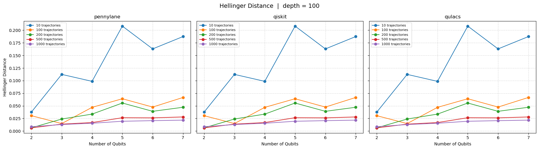
3. Hellinger Distance: Provides a measure of the geometric difference between two probability distributions and is bounded between \([0,1]\), where a value of \(0\) indicates a similar distribution. The value for two discrete distributions can be computed using the equation below. \begin{equation*} HD(p,q) = \frac{1}{\sqrt{2}} \sqrt{\sum_{i=1}^{N}(\sqrt{p_i} - \sqrt{q_i})^2} \end{equation*}

4. Jenson-Shannon (JS) Divergence: It is the smoothed, symmetric version of the KL divergence, measuring the average information divergence between the two distributions and is bounded between \([0, \text{log}(2)]\) where lower the value the lesser the information loss. The value for two discrete distributions can be computed using the equation below. \begin{equation*} JSD(p||q) = \frac{1}{2}(KL(p||m) + KL(q||m)) \text{ with } m = \frac{p+q}{2} \end{equation*}

\begin{equation*} KL(a||b) = \sum_{i=1}^{N}a_i\text{log}(\frac{a_i}{b_i}) \end{equation*}

def compute_metrics(pd_1, pd_2):
    battacharyya_coefficient = np.sum(np.sqrt(pd_1 * pd_2))
    battacharyya_distance = -np.log(battacharyya_coefficient)
    hellinger_distance = np.sqrt(np.sum((np.sqrt(pd_1) - np.sqrt(pd_2))**2)) / np.sqrt(2)
    m = 0.5 * (pd_1 + pd_2)
    js = 0.5 * np.sum(pd_1 * np.log(1e-10 + pd_1 / m) + pd_2 * np.log(1e-10 + pd_2 / m))
    return (battacharyya_coefficient, battacharyya_distance, hellinger_distance, js)

def plot(data, metric_name, depth):
    metric_list = ["Battacharyya Coefficient", "Battacharyya Distance", "Hellinger Distance", "Jensen-Shannon Divergence"]
    trajectory_list = [10, 100, 200, 500, 1000]
    metric_index = metric_list.index(metric_name)
    solvers = ["pennylane", "qiskit", "qulacs"]

    qubit_list_plot = sorted(set(q for (q, d) in data[solvers[0]].keys()))

    fig, axes = plt.subplots(1, 3, figsize=(18, 5), sharey=True)
    fig.suptitle(f"{metric_name}  |  depth = {depth}", fontsize=14)

    for ax, solver in zip(axes, solvers):
        for traj_idx, n_traj in enumerate(trajectory_list):
            values = [
                data[solver][(q, depth)][traj_idx][metric_index]
                for q in qubit_list_plot
                if (q, depth) in data[solver]
            ]
            qubits_available = [q for q in qubit_list_plot if (q, depth) in data[solver]]
            ax.plot(qubits_available, values, marker="o", label=f"{n_traj} trajectories")

        ax.set_title(solver)
        ax.set_xlabel("Number of Qubits")
        ax.set_xticks(qubit_list_plot)
        ax.legend(fontsize=8)
        ax.grid(True, linestyle="--", alpha=0.5)

    axes[0].set_ylabel(metric_name)
    plt.tight_layout()
    plt.show()

def run_experiment(circuit, qubits, depth, log):
    metrics_identifiers = ["Battacharyya Coefficient", "Battacharyya Distance", "Hellinger Distance", "Jensen-Shannon Divergence"]
    log.write("====="*20 + "\n")
    log.write(f"Running Circuit with {qubits} qubits and depth {depth}\n")
    p_ref = circuit.run_with_density_matrix(list(range(qubits)))
    p_10t = circuit.execute(qubits=list(range(qubits)), num_trajectories=10)
    p_100t = circuit.execute(qubits=list(range(qubits)), num_trajectories=100)
    p_200t = circuit.execute(qubits=list(range(qubits)), num_trajectories=200)
    p_500t = circuit.execute(qubits=list(range(qubits)), num_trajectories=500)
    p_1000t = circuit.execute(qubits=list(range(qubits)), num_trajectories=1000)
    metrics_10t = compute_metrics(p_ref, p_10t)
    metrics_100t = compute_metrics(p_ref, p_100t)
    metrics_200t = compute_metrics(p_ref, p_200t)
    metrics_500t = compute_metrics(p_ref, p_500t)
    metrics_1000t = compute_metrics(p_ref, p_1000t)
    traj_list = [10, 100, 200, 500, 1000]
    for traj, metric in enumerate([metrics_10t, metrics_100t, metrics_200t, metrics_500t, metrics_1000t]):
        log.write(f"Metrics for MCWF with {traj_list[traj]} trajectories:\n")
        for identifier, value in zip(metrics_identifiers, metric):
            log.write(f"{identifier}: {value}\n")
    log.write("====="*20 + "\n\n")
    log.flush()
    return metrics_10t, metrics_100t, metrics_200t, metrics_500t, metrics_1000t

Define Randomized Test Parameters

Define the range for the number of qubits to use and the total number of single qubit gates per qubit. Note that an entanglement gate is applied to after each single qubit gate (recommended to start with 2 qubits).

qubit_list = [2, 3, 4, 5, 6, 7]
depth_list = [5, 20, 50, 100]

log_qulacs = open("Results_Log_File_qulacs.log", "w")
log_qiskit = open("Results_Log_File_qiskit.log", "w")
log_pennylane = open("Results_Log_File_pennylane.log", "w")
data = {
    "pennylane" : {},
    "qulacs" : {},
    "qiskit" : {}
}
log_files = {
    "pennylane": log_pennylane,
    "qulacs": log_qulacs,
    "qiskit": log_qiskit
}
for qubits in qubit_list:
    for depth in depth_list:
        circuit_list = None
        for solver in ["pennylane", "qiskit", "qulacs"]:
            circuit = QC(
                num_qubits=qubits,
                noise_model=noise_model,
                backend_qpu_type=qpu_type,
                num_trajectories=1,
                num_cores=60,
                sim_backend=solver,
                jsonize=True,
                verbose=False,
                threshold=1e-4
            )
            if circuit_list is None:
                build_random_circuit(circuit, depth, qubits)
                circuit_list = circuit.instruction_list
            else:
                circuit.instruction_list = circuit_list
            metrics = run_experiment(circuit=circuit, qubits=qubits, depth=depth, log=log_files[solver])
            circuit.shutdown()
            data[solver][(qubits, depth)] = metrics
for solver in ["pennylane", "qiskit", "qulacs"]:
    log_files[solver].close()

plot(data, "Hellinger Distance", depth=100)

---

Download this Notebook - /theory/verification/method_verification.ipynb